Julia: 17X Faster than Python's Scipy, and Easier Too!

Nobody expects good performance from native Python, but we do expect it when calling compiled functions in libraries like Scipy... However, is this really the case?
I’ve been a serious Julia enthusiast for more than two years now. However, I neve try to impose this preference to the people a work with.
Most importantly, my reason not to insist on Julia, is that there is an undeniable influence of the job market in people’s choice of programming languages, and that is an area where Python or C++ experience can pay dividends, and for the time being, Julia apparently cannot.
So sometime, when coding with others, I am led to use Python. This leads to some moments I consider funny, where we meet problems with dependency management, having to rely on explicit type conversions because code is not generic, and of course, dealing with poor performance, all of which could be easily solved in Julia.
This post is about one of such moments.
Performance using Python’s compiled libraries
Now, people expect poor performance when it comes to native Python, but good (or even excellent) performance when you are calling compiled libraries.
One of such libraries, perhaps one of the most popular ones, is Scipy. For the most part, it consists of wrappers to some good-old Fortran and C code written decades ago.
Now, what happens when you need to compose two functions from Scipy? We should get good performance, right? After all, Python is this excellent glue language, and we need to compose two compiled functions written in the same library.
However, since I had run a Numba vs Julia performance benchmark, I knew that trying to compose two different functions compiled with Numba can be actually worse than native Python. So composition and computational performance are no trivial matters.
So what happens when we try to combine Scipy’s C and Fortran functions? Well, let’s see.
Curve fitting and interpolation
Long-story short, we were working with some time-series data that needed to be interpolated at a fixed set of dates. The values of this smoothed and compressed time-series would be then used for clustering, but that is another story.
Now, what is the best algorithm for interpolating noisy data? It’s quite natural to think in terms of curve-fitting, minimizing an error function, with functions that are set to be sufficiently smooth.
In (so-called) non-parametric statistics, there is a method called smoothing splines, where you pick a smoothing parameter , a set of weights , and then find a spline function that satisfies
The function can then be evaluated at the required points.
This is fine, and there is a single Fortran library that gets called by Scipy (FITPACK by P. Dierckx), so it’s very fast.
However, this is not the solution to our original problem. In our case, we don’t have a parameter and a set of weights , but something that plays a similar role: the specific dates where we want to interpolate (a fixed number of them).
We thus need to solve: find me the best fitting cubic spline, using the values at given dates as the optimization parameters. In other words:
where is a fixed set of chosen dates.
This can be easily solved by a two-step process, each one solved by calling a different library:
- Define a spline based on the target dates, using an interpolation library.
- Fit the best of such splines to the data, using an optimization library.
This approach is quite direct, and avoids the need of dealing with cumbersome parameters such as or the weights . Moreover, this methods can easily accomodate additional requirements, like restrictions on the possible values of . So it seems it can be an interesting alternative to the traditional approach. And leveraging a package ecosystem that contains spline-interpolation and optimization routines, this is solvable with 4 or 5 lines of code.
Solution using Scipy
Let’s generate some sample noisy data first:
rng = np.random.default_rng()

xdata = np.linspace(0, 2*np.pi, 35)
y = np.sin(xdata) + 0.2 * rng.normal(size=xdata.size)
In the first place, we define a model, for which will use uniformly distributed points as our fixed dates:
def Spline(x, p):
    t = np.linspace(0, 2*np.pi, p.size)
    p = interpolate.CubicSpline(t, p, bc_type = "natural")
    return p(x)
Now, we can use the scipy.optimize.curve_fit function to fit the model:
But in my first attempt I failed to call this function, so I need to check out the API. The curve_fit documentation states that
“The model function must take the independent variable as the first argument and the parameters to fit as separate remaining arguments”.
So that means that I cannot use Spline(x, p) directly, as I had assumed that p would be of type np.array. The Spline function has to be modified a tiny bit.
def Spline(x, *p):
    t = np.linspace(0, 2*np.pi, len(p))
    p = interpolate.CubicSpline(t, p, bc_type = "natural")
    return p(x)
Now we can call curve_fit
p0 = [0.5]*6
popt, pcov = curve_fit(Spline, xdata, ydata, method="lm")
Great, we got our result! Now let’s plot them.
I’m sure we can evaluate our spline with Spline(xdata, popt), right? After getting a nasty error:
ValueError: `x` must contain at least 2 elements.it turns out that the proper incantation is Spline(xdata, *popt).
Now, as for the performance, the average execution time was 0.00436 seconds, which when multiplied by the tens of millions of times that we had do this in our data set, could result about a day of computing time in a single processor.
Of course, having this 4-liner that took potentially a day to run was enticing enough to see if porting it to Julia would improve performance, and by how much.
Solution using Julia
After searching for interpolation and curve fitting packages around a little bit, I opted for DataInterpolations and LsqFit, as both packages are owned by Julia organizations that I know have other good packages (PumasAI and JuliaNLSolvers).
In particular, the example of how to call LsqFit seemed simple enough.
So let’s define our spline:
function Spline(x,p)
    u = LinRange(0,2π,6)
    poly = CubicSpline(p,u)
    return poly.(x)
end
And let’s try to run the optimization with the most intuitive possible code:
xdata = LinRange(0, 2π, 35)
ydata = sin.(xdata) + 0.2 * randn(size(xdata))

fit = curve_fit(Spline, xdata, ydata, p0)
That worked right away, without requiring any type conversions at all like in the Python case. The capabilities of Julia for writing generic code played nicely here, showing that even unrelated libraries can be seamlessly integrated.
Plotting also works, and since Julia 1.9, the notorious “time to first plot” issue has been solved, as plotting takes a fraction of a second now.
After some proper benchmarking, the average execution time was 245 microseconds (0.000245 seconds), so that’s 17.5X faster than Scipy. Or in other words, from one day of computing time, to a little more than an hour.
By the way, you can download the scripts to run the benchmark in this repo.
Discussion
The Julia code was easier to write: I didn’t have to manually unpack the tuple to satisfy an API, and it was 17X faster.
So to me, the picture is the following: Python is a nice and probably very convenient frontend for certain frameworks, but even minor deviations from standardized use of such libraries can hurt performance extremely badly.
Julia, in turn, is a highly dynamic, interactive, and elegant language, where libraries are highly composable with each other, and where we have no performance penalties compared to compiled languages.
It should, however, be noticed that the Julia package I picked for non-linear curve fitting LsqFit, currently has less features than scipy’s curve_fit, for example, in terms of available optimization methods (LsqFit only supports unconstrained problems via Levenberg-Marquardt, and curve_fit can also call other methods which do support constraints).
But I believe it is a minor issue, as it should be much, much easier to add this missing feature to LsqFit (specially now, with Julia’s package extensions) than to try gain a 17X speed-up by rewriting Scipy’s internals in the way that the likes of PyTorch and TensorFlow have accomplished.
What about this new method for smoothing splines?
On the other hand, if you are curious about this particular method for fitting splines using general purpose optimization and interpolation routines, I think this approach we just sketched is interesting for the following reasons:
- It truly doesn’t require parameter tunning.
- Is flexible, as it can accomodate parameter bounds more easily.
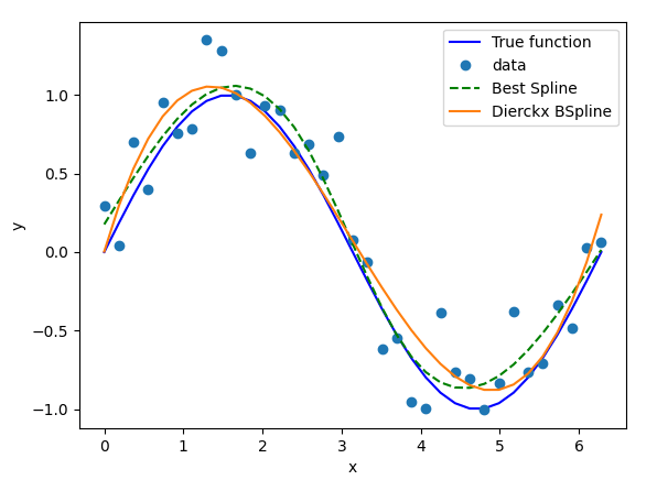
- It turned out to be more accurate than good-old FITPACK, using , available in Scipy as
splrep.
Actually, this were the results of a Montecarlo experiment of fitting a noisy sinusoidal:
| Method | Average Residual error | Average True error | Computing time |
|---|---|---|---|
| splrep | 0.415 | 0.157 | 163 secs |
| Best Splines | 0.401 | 0.106 | 243 secs |
Also, the optimization approach could be valuable for some other use cases: robustness issues with FITPACK come to mind, which could be tackled more easily in the context of general-purpose optimization (i.e. fitting a different objective function other than least squares).
So I believe this shows enough promise for the time it took me to code (very little). And as you see, the performance of my 4-liner Julia code came very close to that of a verenable Fortran library. The Python story would have been very different and very dissapointing in terms of performance, in return for a small gain in precision.
By the way, you can also check this out by running the code in the repo.
Update
Funny enough, I was basing my timings of FITPACK using Python. I was thinking to myself: ok, there is no library composition here, so the timings of splrep should be roughyl equal to that of the original Fortran library.
Silly me, in my test I am also choosing the parameter (which is a part of the method) using a robust scale estimator, the Median Absolute Deviation (MAD), available in scipy.stats.
The MAD can be implemented in 2 lines of code (plus error and NaN handling), or even in a single line of code. I believe that’s why it was so tempting for the authors of scipy.stats to include a “pure python” implementation of it. Not surprisingly, the timings for the computation of absolutely dominate that of the call to the Fortran libray, which is ridiculous.
So this proves two things.
In the first place, no, regrettably my idea for fitting smooth splines is not comptetitive in performance with FITPACK. Altough it is more accurate and flexibe, 87% of the computation time was spent on computing the MAD with Scipy, so the timings above present an unfair comparison.
The other thing it proves (at least, to me) is not that “it is expensive to compose function calls with Python” but rather that Python in a minefield performance-wise. In practice, there is no way to avoid calling some “pure python” one-liner that will cripple performance.
Final toughts
In any case, this quick experiment confirmed to me that Julia is very likely the best language for doing the kind of computational research that I normally do, in terms of performance and productivity.
Its not only 17X faster than scipy, it’s also easier to use, thanks to generic programming.
Of course, I will personally continue to collaborate with people that use either Python or C++ (especially if they have sound reasons like concerns of employability outside of academia).
But I will also continue to rant on this blog whenever I encounter this kind of shortfalls, like having to manually convert between data types, or finding that performance is severely degraded when composing two compiled functions from the same library.