Testing Julia: Fast as Fortran, Versatile as Python

I'm super enthusiastic about Julia after running this comparison of Julia vs Numpy vs Fortran, for performance and code simplicity.

Julia is a pretty new language, which, among other things, aims to solve the so-called “two-language problem” in scientific computing.
That is, we usually test ideas in a rapid-prototyping language like Matlab or Python, but when the testing is done, and its time to do some serious computation, we need to rely on a different (compiled) programming language.
Many tools exist to ease the transition. For example, I have been wrapping up some Fortran into Python via F2PY, which seems like a very convenient way to use (and distribute) efficient Fortran code that anybody can run.
Now, Julia aims to solve this issue in a radical way. The idea is to use a single programming language, which has both an interactive mode, suitable for rapid prototyping, but which can also be compiled and executed at C/Fortran performance.
Code readability: manual vectorization vs simple loops
Opinions on code readability are, of course, subjective. However, I want to explain why I think Numpy doesn’t offer the best quality experience in terms of code clarity.
So far, interpreted languages have required manual re-writing of loops as vector operations. With some practice, this becomes and easy task, but after having done so extensively for many years (first in Matlab, then in Python), I came to the conclusion that I hate to manually vectorize code. I prefer to write for loops and have the compiler vectorize them for me!
Consider the following Numpy code, for example.
n = len(a)
M = np.exp(1j*k*sqrt(a.reshape(n,1)**2 + a.reshape(1,n)**2)
Can you tell what it does, at first sight? Can you reason about the code’s performance? Can you even guess the dimension of the output M? Hint: we are exploiting the fact that, by default, Python will add a matrix and a matrix into an matrix.
Now, here is a nested for loop which does the same as the above code.
for j ∈ 1:n, i ∈ 1:n

    M[i,j] = exp( im*k * sqrt( a[i]^2 + a[j]^2 ) )

end
And here is the mathematical formula it represents:
The Julia syntax is a lot closer to the math. As for loops are fast, we don’t have to worry much about vectorization or anything like that, which takes more time to write, and is obfuscating what the code does.
So even though I fully agree with the idea than Python is a beautiful language to work with, I don’t think the same holds for addons such as Numpy.
Yes, Numpy allows us to stay within a Python framework and get things done with simple one-liners (which is pretty neat anyway) but the resulting Numpy code is much harder to read than a simple loop, even in this extremely simple example.
When we need to vectorize more complicated expressions, and there are no clever shortcuts available, we need to resort to Numpy functions like np.tile which will make the code look like this:
n = len(a)
M = np.exp(1j*k*sqrt(np.tile(a,(n,1))**2 + np.tile(a.reshape(n,1),(1,n))**2))
which is yet another version of the above code.
Personalized micro-benchmarks
I believe there is no such thing as a definitive benchmark. Running a series of completely unrelated tests of toy problems, and claiming that a certain language is overall the best because it does well in most of the tests, is meaningless if we are interested in certain specific and more realistic cases.
Rather than trying to rely on big, all-purpose benchmarks, I believe it is preferable to run, from time to time, some micro-benchmarks suited to our own projects.
If we can predict what the major performance bottlenecks of our code will be,then come up with a minimalistic, but spot-on example, and create a specific performance test that suits our needs.
In my numerical projects, for example, I do a lot of array operations and I evaluate a lot of complex exponentials. So that’s why this test is about just that.
My benchmark was already described above, it’s just: given a vector a, form the matrix
Basic performance tests
As a first test, I opted for out-of-the-box minimalistic codes in each language.
So I wrote a Julia version with no package dependencies whatsoever, and a Fortran code which I could call from Python by wrapping it using F2PY.
| Language | Ease/readability | Lines of code | ST time | MT time |
|---|---|---|---|---|
| Numpy | Very good | 15 | 6.8s | X |
| Basic Julia | Excellent | 21 | 3.0s | 0.6s |
| F2PY-Fortran | Very good | 42 | 4.8s | 1.3s |
Note: ST and MT stand for single-threaded and multithreaded, respectively.
Some quick comments:
- Numpy is restricted to single-threading in many cases, it requires to manually vectorization of code which can become hard to read, and is much slower than the two alternatives.
- Fortran offers great performance with pretty simple code. However, some wrapping is required to call Fortran from high-level languages like Python, which can result in a degraded performance or considerable extra work.
- Julia is faster and easier to write than Numpy’s vectorized code, and it’s significantly faster than F2PY-wrapped Fortran code.
Honestly, I was shocked by what I found in this comparison. I was willing to give Julia a try even if that meant sacrificing a tiny bit of performance, but it seems that there is no need for such a compromise. Julia is amazing.
The complete source code of the tests can be found in this Github repository. The repository includes both basic implementations, and highly-optimized codes. The repository also includes additional ways to speed up Python like Cython, and Numba, for now.
But before getting into such details, let’s review the most basic version of this test (i.e. those that use the simplest possible code and the most convenient setting).
Basic Numpy vs Julia vs F2PY-Fortran Tests
Here is the most basic shared-memory-parallel Julia code for this problem:
function eval_exp(N)
    a = range(0, stop=2*pi, length=N)
    A = Matrix{ComplexF64}(undef, N, N)

    @inbounds Threads.@threads for j in 1:N
    for i in 1:N
        A[i,j] = exp((100+im)*im*sqrt(a[i]^2 + a[j]^2))
    end
    end

    return A

end

eval_exp(5)
print(string("running loop on ", Threads.nthreads(), " threads \n"))
for N in 1000:1000:10000
    @time begin
    A = eval_exp(N)
    end
end
I got the following test results:
| N | Numpy | Fortran ST | Julia ST | Fortran MT | Julia MT |
|---|---|---|---|---|---|
| 1000 | 0.114 | 0.048 | 0.035 | 0.035 | 0.007 |
| 2000 | 0.204 | 0.191 | 0.126 | 0.054 | 0.031 |
| 3000 | 0.448 | 0.421 | 0.289 | 0.117 | 0.062 |
| 4000 | 0.778 | 0.756 | 0.554 | 0.205 | 0.116 |
| 5000 | 1.229 | 1.173 | 0.831 | 0.317 | 0.215 |
| 6000 | 1.741 | 1.686 | 1.108 | 0.456 | 0.274 |
| 7000 | 2.671 | 2.283 | 1.489 | 0.614 | 0.304 |
| 8000 | 4.190 | 2.994 | 1.948 | 0.884 | 0.402 |
| 9000 | 5.319 | 3.797 | 2.460 | 1.022 | 0.505 |
| 10000 | 6.847 | 4.895 | 3.039 | 1.353 | 0.616 |
Notes:
- In all cases, the fast-math optimization flag was used, which allows compilers to reorder mathematical expressions to obtain accuracy, but in a way that could break IEEE compliance.
- This Fortran code was compliled with gfortran and wrapped into Python via F2PY.
- All tests were run in an Intel i7-4700MQ CPU (3.40 GHz, 6MB of Cache) with 8 GB of DDR3 RAM.
Multithreading efficiency
Interestingly, from the above table, we can compute the threading efficiency, which is the speed-up factor when moving from single-threaded to multi-threaded.
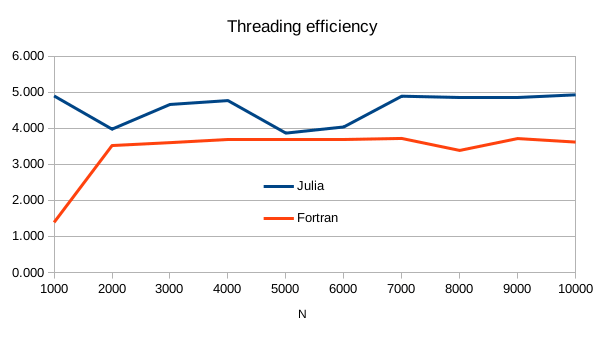
In a quad-core CPU, Julia’s native multithreading efficiency is about 4.9, whereas when relying on gfortran and OpenMP, we get about 3.6. So Julia is effectively taking advantage of hyperthreading, something which is rarely seen in OpenMP.
| N | 1000 | 2000 | 3000 | 4000 | 5000 | 6000 | 7000 | 8000 | 9000 | 10000 |
|---|---|---|---|---|---|---|---|---|---|---|
| Fortran | 1.389 | 3.520 | 3.601 | 3.682 | 3.701 | 3.697 | 3.717 | 3.386 | 3.714 | 3.618 |
| Julia | 4.897 | 3.976 | 4.660 | 4.769 | 3.866 | 4.036 | 4.890 | 4.844 | 4.866 | 4.928 |
Highly Optimized Fortran vs Optimized Julia Performance
The performance story doesn’t end up here. Lets start by considering some improvements on the Fortran side, first, and then on the Julia side.
F2PY vs standalone gfortran
As it has been pointed out to me in the Fortran forum, there can be a significant overhead when calling Fortran from Python via F2PY, when compared with a standalone Fortran code. In this case there was a 50% overhead.
This is not necessarily related to the program spending time at the interface (actually, the F2PY performance report shows only 10% of the time being spent there) but there is perhaps a more fundamental limitation of mixed-language programming going on here.
As the code we compile is larger, the compiler will have a shot at doing some interprocedure optimizations, while when we call a compiled function from a scripting language there is not such possibility.
So, in order to improve the performance on the Fortran side, we must resort to standalone Fortran code. This version has 10 extra lines of code with respect to the F2PY version, and this comes at the additional cost of resigning interoperability with Python.
The importance of being able to easily wrap Fortran code into Python cannot be understated, given the huge ecosystem of I/O libraries, user interfaces, web interfaces, and high-level language features that become available to Fortran programmers when calling their specialized number-crunching code from Python.
GCC math vs Intel’s MKL
The choice of compilers and math libraries can also have a significant effect on performance. In particular, we can get a further 2X speed-up when relying on Intel’s MKL for fast vector math.
This however comes at the cost of some extra 20 lines of code with complicated syntax, graciously contributed by Clyrille Lavigne. MKL can be either wrapped up into F2PY or used for the standalone version.
The main loop now loos like this:
    !$OMP PARALLEL DO DEFAULT(private) SHARED(a_pow_2, M, n, rimk,iimk)
    do j=1,n

    rtmp = a_pow_2 + a_pow_2(j)
    call vdsqrt(n, rtmp, rtmp)

    ! real part
    call vdexp(n, rimk * rtmp, tmp_exp)

    ! imag part
    call vdsincos(n, iimk * rtmp, sinp, cosp)

    ! assemble output
    M(:, j) = cmplx(tmp_exp * cosp, tmp_exp * sinp)
    end do
    !$OMP END PARALLEL DO
Julia vs Intel’s MKL: enter LoopVectorization.jl
The Julia ecosystem has several packages to increase performance beyond straightforward use of the Julia base as I had done so far. One of such packages is LoopVectorization.jl.
Relying on the following code (shared by Mason from the Julia forum) will produce a further 2X speed-up vs the basic Julia version.
function eval_exp_tvectorize(N)
    a = range(0, stop=2*pi, length=N)
    A = Matrix{ComplexF64}(undef, N, N)

    _A = reinterpret(reshape, Float64, A)
    @tvectorize for j in 1:N, i in 1:N
        x = sqrt(a[i]^2 + a[j]^2)
        prefac = exp(-x)
        s, c = sincos(100*x)

        _A[1,i,j] = prefac * c
        _A[2,i,j] = prefac * s
    end
    return A
end
Importantly, the the compromise needed in code clarity for this additional 2X performance gain looks minimal.
Moreover, as LoopVectorization.jl is expected to offer direct support for complex numbers at some point in the future, the syntax for this example could be eventually made just as simple as the one from original basic version.
It is remarkable that this further optimized Julia code is almost exactly as fast as a highly-optimized standalone-Fortran version linked with Intel’s MKL.
Summary
Let’s look at the numbers.
| Language | Ease/readability | Lines of code | MT time |
|---|---|---|---|
| Standalone gfortran | Regular | 52 | 0.87s |
| MKL-gfortran | Regular | 75 | 0.37s |
| LoopVectorization.jl | Very good | 25 | 0.38s |
After going down the performance rabbit-hole, we ended up with a highly-optimized Fortran code which is 75 lines long (compared to 25 in Julia), and it’s not interoperable with Python. This looks like a very high cost to pay for a code that gets the exact same performance. In turn, the Julia version already integrates with a huge ecosystem of open-source libraries.
Preliminary conclusions
Running personal benchmarks to decide which stack is convenient for each use case can be a valuable thing to do, from time to time.
Other things to consider are:
-
We could also resort to the various accelerator libraries available for making Python fast, such as Cython and Numba, as opposed to using Julia or F2PY. Some of this test codes have been contributed to the repository, but I haven’t had time to add some discussion around those topics.
-
Commercial compilers like Intel’s oneAPI might offer slightly better performance, of around 20% or so. More testing is underway on this regard. However, it has to be noted that Intel’s oneAPI, although free for personal use, is a closed-source software with a restrictive license. A paid “concurrent” license might be needed for some use cases related to cloud usage. On this regard, the oneAPI’s fact-sheet states that: “Intel’s gold oneAPI product is free for developers to use locally or in the Intel DevCloud”.
In my case, I am only considering Fortran as a part of a two-language solution that includes Python. In the future, LFortran will likely become a real alternative.
In the meantime, Julia does look like a great option, at least for my use case. I also find the permissive open-source license much desirable, as well.
I will be uploading more benchmark cases to the Github repository, in particular to dig deeper into the various alternatives for making Python fast. If you want to contribute to the testing, you are more than welcome!
If you want to get started coding in Julia, you can also check out a series of posts I’m writing: Numerical Computing in Julia: A Hands-On Tutorial.