Solving Linear Systems

Linear system of the form $Ax = b$ are ubiquitous in engineering and scientific practice.

After the modelling is done, and a discretization strategy is selected, we are usually left with matrix computations.

We often arrive at large systems of linear equations when a continuous problem is discretized. In such cases, the dimension of the problem grows with the need of representing then fine-scale features present in a given physical model.

Example Problem

As we all learn by example, let’s focus on a classical Laplacian problem in one dimension:

Let’s consider now a discrete mesh consisting of $m + 1$ equally-spaced points in the interval $[0,1]$ including the boundaries:

For each point $x_j$ of the mesh, discretizing the second derivative operator $U_{xx}$ using centered differences results in:

Employing the boundary conditions $u_0 = \alpha, u_{m+1}=\beta$ we obtain the system

where

Initializing the Finite Difference Matrix

Now let’s implement this Linear Algebra problem in Julia.

Let’s begin initializing some values

# Problem definition
α = 1;
β = 1;
f(x) = exp(x)

# Create uniform mesh
m = 1000;                     # Select a value
h = 1/(m+1);                  # Spacing between nodes
x = LinRange(0,1,m+2)         # Note: m+2 because LinRange includes boundaries
x_inner = x[2:m+1];           # Inner nodes where we will solve the equations

For simplicity we will resort to a simple loop that fills in the values in an empty matrix. Importantly, let’s recall that loops are JIT-compiled in Julia, so they are absolutely efficient. Also, getting familiar with loops will allow us to later change our codes to more general cases.

# Function to fill values of tridiagonal matrix
function fillmat!(A)
  for i=1:m
    A[i,i] = -2                 # Diagonal
    if i<m
      A[i,i+1] = 1              # Sup-diagonal
    end
    if i>1
      A[i,i-1] = 1              # Sub-diagonal
    end
  end
end

# Create Undefined Matrix and fill values
A = zeros(m,m)
fillmat!(A)
  
# Create Right-hand side  
F = Array{Float64}(undef,m)  
for i=1:m
  F[i] = h^2 * f(x_inner[i])
end
F[1] = F[1] - α
F[m] = F[m] - β

Not that, for notational convenience, we have multiplied both sides of our linear system by $h^2$.

Now we are ready to solve our linear system.

Solve Using Backslash

The first thing we want to do is simply using the built-in standard solver, and get a solution. This is accomplished with the backslash operator.

u = A\F;

As this is a simple test problem, we can also check the accuracy of our method by comparing against an exact solution.

a = - exp(0) + α;
b = β - a - exp(1);
u_exact(x) = exp(x) + a + b*x

We can make this comparison with a simple plot.

using Plots

plot(x,u_exact.(x),marker=8, markeralpha=0.1, label="Exact Solution",legend=:outertopright)
plot!(x,[α; u; β],marker=4, label="Numerical Solution")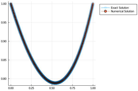

LU Decomposition

Given a system of linear equations:

the LU decomposition of $A$ is such that $PA=LU$, for an upper-triangular matrix $U$, a lower-triangular matrix $L$, and a permutation matrix $P$.

The LU decomposition can be viewed as the matrix form of Gaussian elimination. Finding the LU decomposition of a matrix has a cost of $O(n^3)$ operations.

Interestingly, once we have the LU decomposition, we can apply the following procedure to solve $Ax = b$.

Given $Ax = b$ and $PA=LU$, we have:

This leads into a two-step algorithm to solve this linear system:

• Solve $Ly = Pb$ for $y$,
• Solve $Ux = y$ for $x$.

As $U$ and $L$ are triangular, these operations will have a $O(n^2)$ cost, when applying the algorithms known as back and forward substitution.

For this reason, whenever we need to repeatedly solve linear systems with the same matrix but multiple right-hand sides, for efficiency, we usually precompute the LU decomposition.

Let’s see how we can implement this in Julia.

We can perform a LU factorization of a matrix, and store the result in a variable called lufact, which will have 3 components:

using LinearAlgebra
lufact = lu(A);                 # LU factorization
lufact.L
lufact.U
lufact.p

Alternatively, we can automatically unroll the result, by doing

using LinearAlgebra
L,U,p = lu(A);                  # Unrolling the result

In order to solve this system when given a LU-decomposed matrix, the LinearAlgebra package will apply efficient back and forward substitution operations by default.

luA = lu(A);          
x = luA\F;

It worthwhile to comment about how such functionality is implemented within the LinearAlgebra package.

In particular, there is a “solve” function (the backslash operator) such which acts differently on different types of input. Indeed, the output of lu is a custom type (in other languages we would use the term “object”).

typeof(luA)

LU{Float64, Matrix{Float64}}

We will be discussing these kind of language features in a future post, or more precisely, as we encounter them in our numerical computing journey.

As for timings, I’ve added some simple lines to profile the different methods, like this:

@time begin
# Lines of code you want to time
end

Step	Timing
A\F	0.011587 seconds
LU	0.011954 seconds
LU-solve	0.000661 seconds

As we can see, the cost of doing an LU decomposition is roughly the same as using the backslash operator to solve a linear system, but in this way, each solution $x$ for an extra right-hand side will have a negligible cost when compared with a single solve.

In the future, we will also cover how to profile code more systematically, with various tools offered in the Julia ecosystem.

Sparse matrices

For very large matrices with lots of zeros, we might need to store only the non-zero entries. The SparseArrays.jl package provides an implementation of the necessary operations for such matrices.

using SparseArrays

How to initialize a sparse matrix

The simplest way of initializing a sparse matrix is by converting a dense matrix into a sparse one, by doing:

A = zeros(m,m)
fillmat!(A)
As = sparse(A);                 # m×m SparseMatrixCSC{Float64, Int64}

However, this is also very inefficient.

Creating an empty sparse matrix of zeros, and filling values one by one is a better alternative:

As = spzeros(m,m)
fillmat!(As)

The most efficient ways of initializing a sparse matrix, however, requires to build the corresponding vectors of indices and values, and calling the sparse constructor only once.

In our test case, we would do:

function get_vectors(m)
  II,JJ,V = [Array{Float64}(undef,0) for _ in 1:3]
  for i=1:m
    push!(II,i); push!(JJ,i); push!(V,-2); 
    if i<m
      push!(II,i); push!(JJ,i+1); push!(V,1);   # Sup-Diagonal
    end
    if i>1
      push!(II,i); push!(JJ,i-1); push!(V,1);   # Sub-Diagonal
    end
  end
return II,JJ,V
end

II,JJ,V = get_vectors(m)
As = sparse(II,JJ,V)

As for timings, I’ve arrived at the following:

Method	timing	speed-up
Naive	0.002431 seconds	1
spzeros	0.000646 seconds	3.76
vectors	0.000154 seconds	15.78

Clearly, dealing with sparse matrices requires some extra care, for optimal performance.

LU Factorization of Sparse Matrix

We can do an LU factorization of a SparseMatrixCSC object, by resorting to the LinearAlgebra.jl package. Julia will be internally calling the UMFPACK library.

For exmple, let’s just run

using LinearAlgebra
luAsp = lu(As);                  
x = luAsp\F;

As for timings, this is what I got in my PC:

Method	Timing	Speed-up
Dense-LU	0.010652 seconds	1
Sparse-LU	0.000063 seconds	13

We see that, in the present test case for m=1000, the sparse LU-solve is 13X faster than the dense-matrix version of the same back-substitution routines.

Iterative methods

Another alternative for very large matrices is to rely upon iterative solvers.

Iterative solvers are also very useful in cases where it is possible to speed up the application of $Ax$ for any given vector $x$, without explicitly constructing the matrix $A$.

The IterativeSolvers.jl package contains a number of popular iterative algorithms for solving linear systems, eigensystems, and singular value problems.

using IterativeSolvers

For solving our example problem, we will be relying on GMRES, a general purpose iterative solver of linear systems.

We first need to write a function that computes $Ax$ for any given vector $x$. Given the very simple structure of the matrix under consideration, this can be done quite simply:

iter_A(x) = [ -2x[1] + x[2]; x[1:end-2] - 2x[2:end-1] + x[3:end] ; -2x[end] + x[end-1] ]

It is considered good practice to write “tests” for our numerical routines. In this case we would need to test whether the function iter_A effectively computes the matrix product A*x. We can do so in a simple one-liner:

xt = rand(m);
norm(iter_A(xt)-A*xt)

and check if the result is comparable to machine accuracy. In my case, I get zero or numbers like 4.6 e-21, so I’m confident I didn’t introduce any typos into my function.

Finally, let’s use GMRES to solve this large matrix problem.

The IterativeSolvers packages requires that we define a “LinearMap” satisfying some basic characteristics. Fortunately, we can build this LinearMaps objects from functions like iter_A, with LinearMaps.jl.

using LinearMaps
Ax = LinearMap(x->iter_A(x),m,m)

Finally, for calling unrestarted GMRES with a relative tolerance of 1e-8, we do:

x_gmres = gmres(Ax,F,reltol=1e-8,restart=m)

Note: remember “m” was the dimension of the linear system.

Of course we would like to test this, comparing against the LU solution:

norm(x_gmres-u)
9.606109008315772e-7

For more information, head over to the InterativeSolvers’ Manual.