Linear Least Squares

Least squares models are ubiquitous in science and engineering. In fact, the term least squares can have various meanings in different contexts:
- Algebraically, it is a procedure to find an approximate solution of an overdetermined linear system — instead of trying to solve the equations exactly, we minimize the sum of the squares of the residuals.
- In statistics, the least squares method has important interpretations. For example, under certain assumptions about the data, it can be shown that the estimate coincides with the maximum-likelihood estimate of the parameters of a linear statistical model. Least square estimates are also important even when they do not coincide exactly with a maximum-likelihood estimate.
- Computationally, linear least squares problems are usually solved by means of certain orthogonal matrix factorizations such as QR and SVD.
Computing Least Square Solutions
Given a matrix and a right-hand side vector with , we consider the minimization problem
Solving the Normal Equations
As most linear algebra textbooks show, the most straightforward method to compute a least squares solution is to solve the normal equations
This procedure can be implemented in Julia as:
x = A^t A \ A^t bHowever, this is not the most convenient method from a numerical viewpoint, as the matrix has a condition number of approximately , and can therefore lead to amplification of errors. The QR method provides a much better alternative.
Least squares via QR Decomposition
Another way of solving the Least Squares problem is by means of the QR decomposition (see Wiki), which decomposes a given matrix into the product of an orthogonal matrix Q and an upper-triangular matrix R .
Replacing , the normal equations now read:
Now, given the identity , this expression can be simplified to
For well-behaved problems, at this point we have a linear system with a unique solution. As the matrix is upper-triangular, we can solve for by back-substitution.
In Julia, the least-squares solution by the QR method is built-in the backslash operator, so if we are interested in obtaining the solution of an overdetermined linear system for a given right-hand side, we simply need to do:
x = A\bThere are cases where we want to obtain and store the matrices Q and R from the factorization. An example is when, for performance, we want to pre-compute these matrices and reuse them for multiple right-hand sides. In such case, we do
qrA = qr(A); # QR decomposition
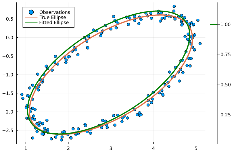
x = qrA\b;Example: Fitting a 2D Ellipse from a Set of Points
Let’s focus in an interesting curve-fitting problem, where we are given pairs of points and we want to find the ellipse which provides the best fit.
There are indeed many ways of solving this curve-fitting problem (see for example this paper.
The most basic method starts with noting that the points of a general conic satisfy the following implicit equation:
The above equation can be normalized in various ways. For example, we can resort to the alternative formulation:
This leads to the problem of finding the best-fitting coefficients as a least-squares problem for the following equations with 5 unknowns:
Let’s generate some random test data
θ = π/7; a = 2; b = 1.5; x_0 = 3; y_0 = -1;
fx(t) = a*cos(θ)*cos(t) - b*sin(θ)*sin(t) + x_0
fy(t) = a*sin(θ)*sin(t) + b*cos(θ)*cos(t) + y_0

N = 200;
ts = LinRange(0,2π,N);
x = fx.(ts) + randn(N)*0.1;
y = fy.(ts) + randn(N)*0.1;
We now construct the design matrix
A = [x.^2 y.^2 x.*y x y ]and compute the least-squares solution with the backslash operator:
p = A\ones(N)Thats it! We have obtained the parameters of the implicit equation.
Plotting the Implicit Curve as a Countour Line
However, if we want to plot the resulting curve, we must solve an additional problem. Given , how can we find points satisfying:
and plot them?
Fortunately, this can be easily accomplished by resorting to contour plots. In order to do this, we construct a grid and we evaluate the (bivariate) polynomial expression field. Then, we seek the contour level equal to one. Under the hood, the plotting code is using the marching squares algoritm.
using Plots
X = LinRange(minimum(x),maximum(x),100)
Y = LinRange(minimum(y),maximum(y),100)
F = Array{Float64}(undef,100,100)
for i ∈ 1:100, j ∈ 1:100
    F[i,j] = p[1]*X[i]^2 + p[2]*Y[j]^2 + p[3]*X[i]*Y[j] + p[4]*X[i] + p[5]*Y[j]
end

plot(x,y,seriestype = :scatter, label="Observations", legend=:topleft)
plot!(fx.(ts), fy.(ts), linewidth=3, label="True Ellipse")
contour!(X, Y, F, linewidth=3, levels=[1], color=:green)
plot!([], color=:green, label="Fitted Ellipse")