Numerical Integration

Numerical integration deals with the approximate evaluation of definite integrals.

Quadrature formulas are needed for cases in which either the anti-derivative of the integrand is unknown, or for which the integrand itself is only available at a discrete set of points. Importantly, quadrature provides a basic tool for the numerical solution of differential and integral equations.

Simple and Composite Quadrature Rules

Midpoint Rule

The most basic integration rule is obtained by approximating the integrand by a constant, and integrating that constant in the interval $(a,b)$. The value of the function at the interval midpoint is often employed.

One possible way to obtain more accuracy is to turn to the composite midpoint rule, which is the same idea behind the definition of the integral as a limit of Riemmann sums. Considering a set of equally spaced points, we then have:

The following shows an example Julia implementation:

function quad_midpoint(f,a,b,N) 
    h = (b-a)/N
    int = 0.0
    for k=1:N
        xk_mid = (b-a) * (2k-1)/(2N) + a
        int = int + h*f(xk_mid)
    end
    return int
end

Trapezoidal Rule

A more accurate variation of the midpoint rule is the trapezoidal rule, which uses the information of the values of the function at two points in each interval. In this case, in each interval $a,b$ we approximate the integrand by a linear function, and we integrate that linear function exactly. That procedure leads to the following expression:

The composite trapezoidal rule, for the case of equally-spaced points $x_j = hj + a, j=0,...,N$, with $h = (b-a)/N$, then reads:

This can be implemented in Julia with the following code:

function quad_trap(f,a,b,N) 
    h = (b-a)/N
    int = h * ( f(a) + f(b) ) / 2
    for k=1:N-1
        xk = (b-a) * k/N + a
        int = int + h*f(xk)
    end
    return int
end

Quadrature of Smooth and Periodic Functions

A particular case of interest is that of smooth and periodic functions. In this case, the composite Trapezoidal Rule converges exponentially fast, which can be counter-intuitive.

Let’s illustrate this with the following example. We will integrate a smooth and $2\pi$-periodic function with the trapezoidal rule.

using Printf
f(x) = exp(cos(x)^3)
ref = quad_trap(f,0,2π,10000);

for n=2:5
    error = abs(quad_trap(f,0,2π,2^n) - ref)
    @printf("n=%3i, %4.2e\n", 2^n,error)
end

n=  4, 6.64e-01
n=  8, 9.02e-03
n= 16, 1.40e-06
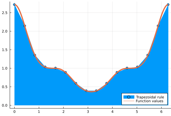
n= 32, 6.22e-15

To see how this actually looks like, let’s generate a picture of the function and it’s approximation,, which we can do with the following code:

x_true = LinRange(0,2π,1600)
x_trap = LinRange(0,2π,16)
plot(x_trap,f.(x_trap),fillrange=0,label="Trapezoidal rule")
plot!(x_true,f.(x_true),line=4,legend=:bottomright,label="Function values")

Remarkably, even though the local errors in the trapezoidal rule approximation of the area beneath the curve are clearly visible, the global result is correct to the 6th decimal place!. The picture was generated with the following code:

Newton-Cotes Rules

The ideas of the previous methods can be generalized to higher orders of accuracy. That is, the integrand can be approximated by higher order polynomials. However, we should remember that interpolation on equally spaced points suffers from the Runge phenomenon. So in practice, Newton-Cotes rules will be limited to low degree polynomials.

Gauss-Kronrod Adaptive Quadrature with QuadGK.jl

The QuadGK.jl package implements adaptive Gauss-Kronrod quadrature. Adaptive quadrature comes into play when we want high accuracy for general types of functions, whose characteristics are unknown a-priori.

As a test case, let’s try to integrate the square root function with 8 digits of accuracy.

using QuadGK
f(x) = sqrt(x)
a=0
b=1
I,est = quadgk(f, a, b, rtol=1e-8)

(0.6666666668118825, 2.5136408476444087e-9)

quadgk returns a pair $(I,est)$, where $est$ is an error estimate.

Fast Gaussian Nodes and Weights with FastGaussQuadrature.jl

For the cases in which we know beforehand that our function is smooth, using higher order Gauss-Legendre rules should be substantially more efficient than relying on adaptive quadrature.

The FastGaussQuadrature.jl package implements fast algorithms to compute sets of nodes and weights $x, w$ in $O(n)$ time.

using FastGaussQuadrature
@time x, w = gausslegendre( 10_000_000 );

0.318357 seconds (10 allocations: 228.882 MiB)

That’s 10 million Gauss-Legendre quadrature nodes and weights computed in a fraction of a second.

Actually, Gauss quadrature is so accurate for smooth functions that we rarely need so many points. For a very simple integration problem like $\int_{-1}^1 e^{t} dt$, even 7 points already yield full machine precision:

x, w = gausslegendre( 7 );
exact = exp(1)-exp(-1);
numer = w'exp.(x);
abs(numer-exact)

8.881784197001252e-16

Double Integrals

Let’s compute a double integral:

One of the simplest, and most efficient ways of coding this is by resorting to Gauss-Legendre quadrature. Simply compute the weigths and, by virtue of Fubini’s theorem, apply the quadrature rule in each variable. This can be implemented as follows:

f(x,y) = exp(-(x^2+y^2))

function Quad2D(f,n)
    x, w = gausslegendre( n );
    y = x;
    sum = 0
    for i=1:n, j=1:n
        sum = sum + f(x[i],y[j]) * w[i] * w[j]
    end
    return sum
end

In this case, we only need $n =12$ to get 14 digits of accuracy.