Polynomial Interpolation

We describe some basic approaches for polynomial approximation, and how to implement them in Julia.
Polynomials are one of the simplest yet more powerful objects in mathematics. They are very convenient to use for numerical purposes, as they are based on just additions and multiplications. Trying to use polynomials for the approximation of complicated functions seems a very desirable goal to achieve.
A classical approach to polynomial interpolation is to specify points at which a polynomial of degree should match a given function.
Another approach we will discuss is that of interpolation by splines, that is, piecewise polynomial approximation. Given the flexibility of this approach, it is employed very often in many areas of numerical computing.
Interpolation is not only important as a tool to approximate complicated but well-known functions. It can also be employed to approximate the solution of important problems in physics and engineering, such as the solution of differential and integral equations.
The Vandermonde Matrix
A polynomial in the canonical basis (or power form) is given by
The coefficients of a polynomial which satisfies the interpolation conditions on a certain mesh , can be expressed as the solution of the linear system
The matrix appearing in this linear system is known as the Vandermonde matrix of the mesh .
This method is rarely used in practice because the Vandermonde matrix is highly ill-conditioned.
The Barycentric Lagrange Interpolation Formula
The barycentric form of Lagrange polynomial interpolation is a fast and stable method, that should probably be known as the standard method of polynomial interpolation.
Let’s consider grid , and let’s try to obtain the polynomial such that
It is easy to check that the solution to this problem can be written in the Lagrange form:
Importantly, there is a more convenient way to express this solution. The so-called barycentric Lagrange form is given by:
where the barycentric weights are given by:
The story doesn’t end here. Interestingly, there are explicit formulas for the barycentric weighs in many important cases.
For example, for equidistant points in an interval , after cancelling factors independent of j (which won’t affect the value of ) we have:
Lagrange Interpolation Algorithm
Given an explicit set of barycentric weights, Lagrange interpolation can be implemented as follows:
function LagrangeInterp1D( fvals, xnodes, barw, t )
    numt = 0
	denomt = 0

	for j = 1 : length( xnodes )
		tdiff = t - xnodes[j]
		numt = numt + barw[j] / tdiff * fvals[j]
		denomt = denomt + barw[j] / tdiff

		if ( abs(tdiff) < 1e-15 )
			numt = fvals[j]
            denomt = 1.0
            break
		end
	end

    return numt / denomt

end
A few examples of sets of points and corresponding weights are the following:
# Equispaced points
EquispacedNodes(n) = [2*(j/n-0.5) for j=0:n]
EquispacedBarWeights(n) = [ (-1)^j * binomial(n,j) for j=0:n ]

# Chebyshev points of the second kind
ClosedChebNodes(n) = [cos(jπ/n) for j=0:n]
ClosedChebBarWeights(n) = [0.5; [(-1)^j for j=1:n-1]; 0.5*(-1)^n]
Equispaced Points: Runge Phenomena
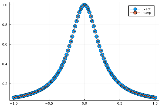
Interpolation at equispaced points can be employed for a small number of points. Let’s consider the following example. We will interpolate the function
f(x) = 1/(1 + 16*x^2)sampled at 15 points. Let’s begin with equispaced points:
using Plots

# Sampling
n = 15;
xnodes = EquispacedNodes(n);
w = EquispacedBarWeights(n);
f_sample = f.(xnodes);

# Interpolation
t = LinRange(-1,1,100)
f_interp = [LagrangeInterp1D( f_sample, xnodes, w, t[j] ) for j=1:length(t)]
plot(t,f.(t), label="Exact", marker = 3)
plot!(t,f_interp, label="Interp", marker = 3)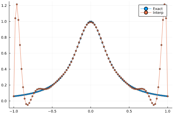
This is a terribly bad approximation. The interpolating polynomial is displaying large oscillatory errors, in what is known as the Runge phenomenon. And it even gets worse with additional interpolation points.
Chebyshev Interpolation Example
The main advantage of Chebyshev interpolation over equispaced points is that we can overcome the Runge phenomenon.
Let’s consider the same function as above, but let’s sample it at 32 Chebyshev nodes of the second kind.
# Sampling
n = 32;
xnodes = ClosedChebNodes(n);
w = ClosedChebBarWeights(n);
f_sample = f.(xnodes);

# Interpolation
t = LinRange(-1,1,100)
f_interp = [LagrangeInterp1D( f_sample, xnodes, w, t[j] ) for j=1:length(t)]
plot(t,f.(t), label="Exact", marker = 8)
plot!(t,f_interp, label="Interp", marker = 3)
Piecewise Polynomial Interpolation
A workaround the Runge phenomena, that will still works on equispaced grids, is to employ piecewise interpolation. That is, relying on low-order interpolants in a finer grid.
While the convergence order is much lower than that of Chebyshev-based interpolation, this method is guaranteed to work for equispaced grids, is fast, and therefore very convenient to use.
Interpolations.jl package
The Interpolations.jl package provides several functionalities for piecewise polynomial interpolation:
- Various extrapolation methods
- Performance-optimized code for cases such as uniform grids
- Linear, Cubic splines
- Multidimensional
In the following test we will display linear vs cubic splines, with linear extrapolation.
using Interpolations
using Plots

# Example data to interpolate
x = LinRange(0,π,5)
y = sin.(x)

# Build Interpolation functions
linear_spline = LinearInterpolation(x, y, extrapolation_bc = Line() )
cubic_spline = CubicSplineInterpolation(x, y, extrapolation_bc = Line())

# Evaluate interpolants and plot results
plot(x,y,marker=5,linetype=:scatter, label = "Data", title = "Piecewise Interpolation Test")

x_ext = LinRange(-0.1,π+1.5,100)
plot!(x_ext, sin.(x_ext), label="Actual Function")
plot!(x_ext,linear_spline(x_ext), label="Linear Spline")
plot!(x_ext,cubic_spline(x_ext), label="Cubic Spline")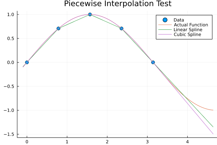
Piecewise Linear Interpolation
Let’s analyze the linear case in detail, which is the simplest case of piecewise interpolation.
As a first step, for a given target point t, we need to find an interval index k such that
To do this, we can resort to the function searchsortedfirst from Julia base, in case we are given a sorted vector x.
k = searchsortedfirst(x, t) # Returns first k such that t <= x[k]We can now define the linear interpolant as a convex combination of the values and .
To do this, we first map the interval to , by defining the following function:
As it is easy to check a linear function that passes through and is then given by:
Putting it all together, we have the following function.
function LinearSpline(x,y,t)
    Y = Array{Float64}(undef,length(t))
    for i=1:length(t)
        k = searchsortedfirst(x, t[i])
        if k <= 1
            k = 2
        elseif k >= length(x)
            k = length(x) - 1
        end
        λ = ( t[i] - x[k-1] ) / ( x[k] - x[k-1])
        Y[i] =  λ * ( y[k] - y[k-1] ) + y[k-1]
    end
    return Y
end
The conditions on k <= 1 and k >= length(x) give rise to linear extrapolation outside of the boundaries of x.
At the time of writing this, this simple function is slightly faster than the corresponding one in Interpolations.jl, for the case of non-uniformly sampled data.
x = LinRange(0,1,400).^2
y = sin.(3x)
t = LinRange(-0.1,1.1,6000)

itp = LinearInterpolation(x, y, extrapolation_bc = Line() )
F(t) = LinearSpline(x,y,t)

@btime itp(t)
@btime F(t)
280.657 μs (2 allocations: 46.95 KiB)
231.245 μs (3 allocations: 47.00 KiB)It is also about 2X slower than the uniformly-sampled case:
x = LinRange(0,1,400)
y = sin.(3x)
t = LinRange(-0.1,1.1,6000)

itp = LinearInterpolation(x, y, extrapolation_bc = Line() )
F(t) = LinearSpline(x,y,t)

@btime itp(t)
@btime F(t)
103.810 μs (2 allocations: 46.95 KiB)
217.207 μs (3 allocations: 47.00 KiB)The reason is that Interpolations.jl is applying an optimized version for the uniformly spaced case (when x is of type LinRange), and in particular, doesn’t need to use the searchsortedfirst function.
This is an expanding tutorial series… stay tuned for more content, and don’t hesitate to contact me if you have any questions.
In particular, we will revisit this case in the future, when we get to discuss performance or other advanced issues in more detail.
References
- [1] Berrut and Trefethen, Barycentric Lagrange Interpolation