Introduction
In many applications, we want to take advantage that the derivative operator is transformed into a multiplication operator in Fourier space. By applying a subsequent inverse transform, we can expect to obtain the derivative of a function using FFTs, using the well-known relation:
However, this is not so simple to translate into the discrete setting.
Common Gotcha: Alising
For example, let’s compute the FFT-derivative of a periodic function defined in . The following code yields an incorrect result:
using FFTW
using plots

N = 20;
L = 1;
xj = (0:N-1)*L/N;
f = sin.(2π*xj)
df = 2π*cos.(2π*xj)

k = 1:N
df_fft = ifft( 2π/L * k.* fft(f) )

plot(xj,real(df),label="Exact derivative")
plot!(xj,real(df_fft),label="incorrect FFT derivative",markershape=:circle)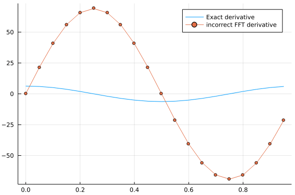
The reason this doesn’t work is related to aliasing, which we discussed in the previous section. In detail, what’s going on under the hood is that, even though in our grid, we have the equality
clearly, the frequency corresponding to k=15 should not be employed when computing the derivative.
The correct derivative algorithm uses the negative frequencies mentioned in the previous section.
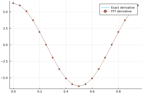
Correct FFT-Derivative Algorithm
In order to obtain the correct result, we to correct these two lines:
k = fftfreq(N)*N;
df_fft = ifft( 2π*im/L * k.* fft(f) );