Using Numpy's FFT in Python

by Martin D. Maas, Ph.D

Last updated: October 30, 2023

There are numerous ways to call FFT libraries both in Numpy, Scipy or standalone packages such as PyFFTW. In this post, we will be using Numpy's FFT implementation.

Definition and normalization

As usual, we want to make sure we get the definition right, as the normalization coefficients or the sign of the exponent can be arbitrary.

As per the official documentation, the DFT is defined as

\begin{equation*} A_k = \sum_{m=0}^{n-1} a_m \exp\lbrace -2\pi i \frac{mk}{n} \rbrace \quad k=0, \dots, n-1 \end{equation*}

while the inverse DFT is defined as

\begin{equation*} a_m = \frac{1}{n} \sum_{k=0}^{n-1} A_k \exp \lbrace 2\pi i \frac{mk}{n} \rbrace \quad m=0, \dots, n-1 \end{equation*}

We can check that this matches the definition we gave in the previous section.

fftshift and fftfreq

In many applications of the FFT, we are not really interested in the raw indices $k$ or $m$ , but rather, on the true frequencies that these indices represent.

In order to obtain those true frequencies, we must shift the zero-frequency component to the center of the spectrum and reorder the coefficients, as we discussed on the previous section along with the almost identical topic of aliasing and negative frequencies, which are a common source of confusion when implementing algorithms that rely on the FFT.

Let’s see how the fftshift function reorders a vector of size N by considering two simple examples, one for an even value of N, and an other for an odd value of N:

import numpy as np
from numpy.fft import fft, fftshift, fftfreq

fftshift(np.arange(0,10))

array([5, 6, 7, 8, 9, 0, 1, 2, 3, 4])

fftshift(np.arange(0,11))

array([ 6,  7,  8,  9, 10,  0,  1,  2,  3,  4,  5])

Another useful function, fftfreq gives the correct frequencies (that is, below Nyquist) that the FFT algorithm is producing. By default, this function will return the frequencies divided by N, so we multiply by N in order to get the shifted indices we desire (see the docs on fftfreq).

N = 10
fftfreq(N)*N

array([ 0.,  1.,  2.,  3.,  4., -5., -4., -3., -2., -1.])

Now lets combine these two functions to compare the original with the shifted indices and coefficients.

import numpy as np
from numpy.fft import fft, fftshift, fftfreq
from matplotlib import pyplot as plt

N = 21
xj = np.arange(0,N)*2*np.pi/N
f = 2*np.exp(17*1j*xj) + 3*np.exp(6*1j*xj) + np.random.rand(N)

original_k = np.arange(0,N)
shifted_k = fftshift(fftfreq(N)*N)

original_fft = fft(f)
shifted_fft = fftshift(fft(f))

fig, axs = plt.subplots(2,1)

axs[0].plot(original_k, np.abs(original_fft))
axs[0].plot([0,6,17], np.abs(original_fft[[0,6,17]]),"o")
axs[0].set_title("Original FFT coefficients")
axs[0].set_xticks(original_k)

axs[1].plot(shifted_k, np.abs(shifted_fft))
axs[1].plot([-4,0,6], np.abs(shifted_fft[[6,10,16]]),"o")
axs[1].set_title("Shifted FFT coefficients")
axs[1].set_xticks(shifted_k)

plt.tight_layout()
plt.show()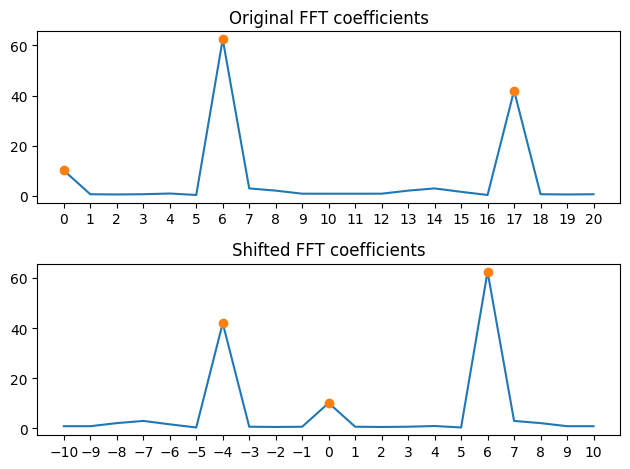

png

Sampling Rate and Frequency Spectrum Example

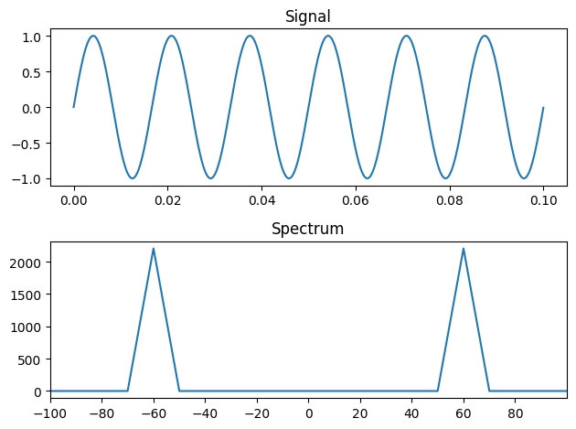
Using the functions fft, fftshift and fftfreq, let’s now create an example using an arbitrary time interval and sampling rate.

We will use a sampling rate of 44100 Hz, and measure a simple sinusoidal signal $sin(60 * 2\pi * t)$ for a total of 0.1 seconds.

import numpy as np
from numpy.fft import fft, fftshift, fftfreq
from matplotlib import pyplot as plt

t0 = 0              # Start time 
fs = 44100          # Sampling rate (Hz)
tmax = 0.1          # End time       

t = np.arange(t0, tmax, 1/fs)
signal = np.sin(2 *np.pi * 60 * t)

F = fftshift(fft(signal))
freqs = fftshift(fftfreq(len(t), 1/fs))

fig, axs = plt.subplots(2,1)
axs[0].plot(t, signal)
axs[0].set_title("Signal")

axs[1].plot(freqs, np.abs(F))
axs[1].set_title("Spectrum")
axs[1].set_xlim((-100, 100))
axs[1].set_xticks(np.arange(-100,100,20))

plt.tight_layout()
plt.show()

png