Using the FFTW Library in Julia

Julia implements FFTs according to a general Abstract FFTs framework. That framework then relies on a library that serves as a backend. In case we want to use the popular FFTW backend, we need to add the FFTW.jl package.

using FFTW

Definition and Normalization

In the previous section we had the following definition for the Discrete Fourier Transform:

in terms of the N-point grid in $[0,2\pi)$ which starts from zero and doesn’t contain the end-point:

In Julia, the Abstract FFTs defines both the DFT and inverse DFT using the following two formulas

Looking at this carefully, and replacing the vector $A[n]$ with $v_j$ for a more readable notation, we can check that this actually coincides with our definition.

fftshift and fftfreq

We can use the fftshift and fftfreq functions to shift the FFT coefficients, in order to obtain the true (below Nyquist) frequencies, that corresponds to each coefficient. You can read more about this in the previous section which included a discussion about aliasing.

Let’s see how the fftshift function reorders a vector by considering two simple examples, one for N even and an other for N odd:

fftshift(1:10)'

 6  7  8  9  10  1  2  3  4  5

fftshift(1:11)'

 7  8  9  10  11  1  2  3  4  5  6

Another useful function, fftfreq gives the correct frequencies (that is, below Nyquist) that the FFT algorithm is producing. Note that the second argument in fftfreq, is the sampling rate (which we are assuming here is equal to N).

N=10
fftfreq(N,N)

 0.0  1.0  2.0  3.0  4.0  -5.0  -4.0  -3.0  -2.0  -1.0

N=11
fftfreq(N,N)

 0.0  1.0  2.0  3.0  4.0  5.0  -5.0  -4.0  -3.0  -2.0  -1.0

Let’s put everything together, and shift our frequencies and coefficients. To do this, we apply the function fftshift to both the fft coefficients, and to the original (below Nyquist) frequencies returned by fftfreq.

using FFTW
using Plots

N = 21
xj = (0:N-1)*2*π/N
f = 2*exp.(17*im*xj) + 3*exp.(6*im*xj) + rand(N)

original_k = 1:N
shifted_k = fftshift(fftfreq(N)*N)

original_fft = fft(f)
shifted_fft = fftshift(fft(f))

p1 = plot(original_k,abs.(original_fft),title="Original FFT Coefficients", xticks=original_k[1:2:end], legend=false, ylims=(0,70));
p1 = plot!([1,7,18],abs.(original_fft[[1,7,18]]),markershape=:circle,markersize=6,linecolor="white");
p2 = plot(shifted_k,abs.(shifted_fft),title="Shifted FFT Coefficients",xticks=shifted_k[1:2:end], legend=false, ylims=(0,70));
p2 = plot!([-4,0,6],abs.(shifted_fft[[7,11,17]]),markershape=:circle,markersize=6,linecolor="white");
plot(p1,p2,layout=(2,1))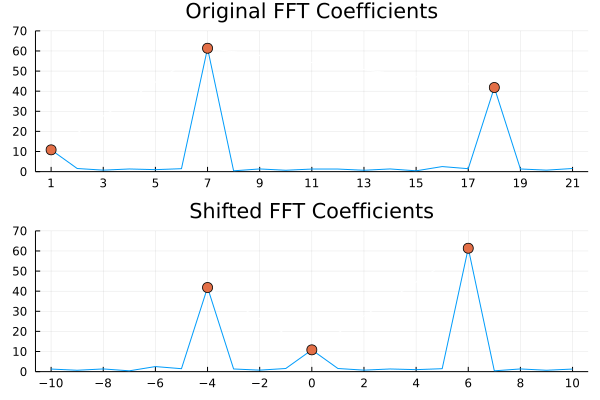

Sampling Rate and Frequency Spectrum Example

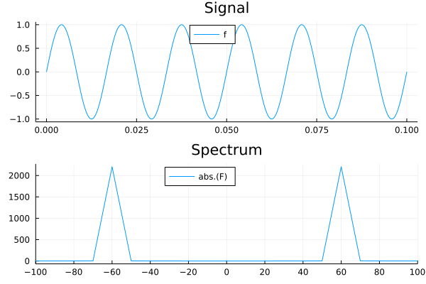
Using the functions fft, fftshift and fftfreq, let’s now create an example using an arbitrary time interval and sampling rate.

We will use a sampling rate of 44100 Hz, and measure a simple sinusoidal signal $\sin(60 * 2 \pi * t)$ for a total of 0.1 seconds.

using FFTW
using Plots

t0 = 0              # Start time 
fs = 44100          # Sampling rate (Hz)
tmax = 0.1          # End time       

t = t0:1/fs:tmax;   
signal = sin.(2π * 60 .* t)

F = fftshift(fft(signal))
freqs = fftshift(fftfreq(length(t), fs))

# plots 
time_domain = plot(t, signal, title = "Signal", label='f',legend=:top)
freq_domain = plot(freqs, abs.(F), title = "Spectrum", xlim=(-100, +100), xticks=-100:20:100, label="abs.(F)",legend=:top) 
plot(time_domain, freq_domain, layout = (2,1))

Performance Tips

Use Real FFTs for Real Data

As we have discussed in the basic properties page, if the input data is real, we can obtain a 2X speedup by resorting the the rfft function.

The function which is slightly harder to grasp is the inverse transform, which we use to to invert the result of rfft. In Julia, we have the irfft(A, d [, dims]) function.

The function irfft requires an additional argument (d), which is the length of the original transformed real input signal, which cannot be inferred directly from the input A.

Let’s make a simple test, where we check if we can indeed transform and back-transform a real signal using rfft and irfft.

using FFTW
using Test

N = 22
xj = (0:N-1)*2*π/N
f = 2*sin.(6*xj) + 0.1*rand(N)
Y = rfft(f)
f2 = irfft(Y,N)

@test f ≈ f2
# Test Passed

Using plans

In case we are going to perform several FFTs of the same size, it is convenient to pre-compute the so-called ‘fft plans’.

The most general (complex-valued) of these functions are: plan_fft, and plan_ifft. An example on how to use plan_fft is:

x=rand(ComplexF64,1000);
p = plan_fft(x; flags=FFTW.ESTIMATE, timelimit=Inf)

As for timings, we can check out that preparaing the plan in this case has produce a 3X speed-up over the basic command.

@time fft_x = p*x;

  0.000029 seconds (2 allocations: 31.500 KiB)

@time fft_x = fft(x);

  0.000093 seconds (34 allocations: 33.922 KiB)  

In-place FFTs (that is, an FFT that modifies the input vector rather than allocating memory and returning a new variable) can be optimized similarly, as well, by doing

p = plan_fft!(x)

Using Intel’s MKL

Intel’s MKL provides a notable implementation of FFT, which is available in Julia via the same FFTW.jl package. To enable it, simply open the Julia REPL and type:

FFTW.set_provider!("mkl")

After restarting Julia and running ‘using FFTW’ again, the required MKL components will be automatically downloaded and installed.