FFT Interpolation and Zero-Padding

Interpolation via Zero Padding

FFT interpolation is based on adding zeros at higher frequencies of the Fourier coefficient vector.

In such way, the inverse FFT will produce more output, using the same non-zero Fourier coefficients.

When implementing this procedure, it’s important to pay attention to the interplay of the normalization constants, the number of points, and the interpolation grid that is being employed, and to make sure that we pad the true high-frequency components of the computed spectrum (i.e. beware of aliasing).

Let’s consider a peridic function in $[0,1]$ evaluated at $N$ equispaced points (not containing the right-endpoint of 1), which we want to interpolate into $Ni$ points.

The following simple test illustrates how to do that.

using Plots
using FFTW

N = 30;   
x = (0:N-1)/N;

Ni = 300; 
xi = (0:Ni-1)/Ni;

f = exp.(sin.(2π*x));
ft = fftshift(fft(f))

Npad = floor(Int64, Ni/2 - N/2)
ft_pad = [zeros(Npad); ft; zeros(Npad)];
f_interp = real(ifft( fftshift(ft_pad) )) *Ni/N ;

plot(x,f, label="Original samples",markershape=:circle)
plot!(xi,f_interp,label="Interpolated values")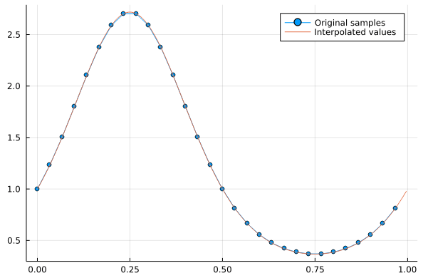

If you want to know more about what fftshift is doing, check out the fftshift section of the introduction to this chapter.

Conclusion

That was a quick glipse of how to implement FFT interpolation in one dimension.

Many more things are possible from here… Let me know in the Reach Out! form below if you would like me to create more content on these topics.