Landsat & Sentinel-2 Data on AWS

by Martin D. Maas, Ph.D

Last updated: July 5, 2022

This post will show you how to leverage cloud-optimized GeoTiffs and the AWS free tier to access satellite imagery, using Python.

Sentinel's NDVI, for Buenos Aires farmland, 12-5-2021.

Working with high-resolution satellite imagery, before the recent development Cloud-Optimized GeoTIFFs (COG), required downloading massive datasets which, most of the time, included a lot of useless data. More often than not, a user wants to access only a few bands in a small area at a time, instead of a full multispectral scene.

With Cloud-Optimized GeoTIFFs, we can now query a web server just for the information we require. This has made working with high-resolution imagery substantially easier (and cheaper, as well!).

You can get the complete code for this tutorial in this repository.

Cost of satellite imagery on AWS

Accessing public datasets on AWS like Landsat and Sentinel are stored in requester-pays buckets. This requires payment for data transfer and processing above the free-tier quotas, which should suffice for prototyping and other use cases, making access to this data virtually free for most use cases.

In detail, AWS always-free tier was recently expanded to 100GB per month of network egress.

What’s important about this is that code can be prototyped for free, downloading data and processing data locally, and deployed into production using AWS services like AWS Lambda, which also have a convenient free-tier.

Other reasons why AWS for Geospatial can be a good suit for many use cases is that:

It leaves freedom regarding the choice of programming languages and libraries you can use.
It allows to rapidly transition from prototyping into production.
Is based on open-source tools which means there is less vendor lock-in.

At least at the time of writing this, none of these seems to be possible with GEE. As I’ve discussed in this post, GEE imposes many restrictions in return for a totally free service, which is comprehensible.

Downloading Sentinel-2 data from AWS

Ok, now that we cleared the convenience of relying on COG on AWS, let’s go about how to actually do this.

Now, we should beware that cloud-native geospatial development is still a rapidly changing field. Not surprisingly, I’ve noticed a certain lack of updated documentation in this area, as I had to go through lots of outdated tutorials to be able to begin working with this new technology.

Step 1: Create and configure an AWS account and the AWS CLI

The first thing you need is an AWS account. Remember that Amazon wants everybody’s credit card information, including users of the free-tier services.

This step has been covered over and over on other places, like here on the AWS site.

You will also need to set up the AWS Command Line Interface. To do so, you can follow this instructions.

Step 2: Find a STAC server and explore collections

Now we need to find which Landsat or Sentinel scenes we are interested in. To do this, another interesting development took place recently, which was the creation of the STAC standard for Spatio-temporal asset catalogs.

As possitive as this recent development might be, regrettably the standardization process seems to be taking some time, with some servers implementing only a portion of the standard, and the existance of certain client/server incompatibility.

The first important thing is to obtain the URLs of actual, functioning, STAC servers. So far, I’ve found the following:

For Sentinel-2, the team of Element84 maintains the earth-search catalog on AWS https://earth-search.aws.element84.com/v0.
For Landsat, we can use the official USGS STAC server https://landsatlook.usgs.gov/stac-server, which includes s3 file locations in their metadata.
For many other collections, the Microsoft Planetary Computer has a STAC server at https://planetarycomputer-staging.microsoft.com/api/stac/v1

To query a STAC server, we are going to have to use two Python packages:

pystac-client for the USGS STAC server. Official docs
sat-search for Sentinel data on AWS’s earth-search.

To install these packages,

pip install pystac-client sat-search

The reason to use two clients is that, at the time of writing this, the earth-search API endpoint we need for the Sentinel data doesn’t seem to be running a server which is compatible with the latest STAC standard, which the more actively developed pystac_client requires. On the other hand, the package sat-search continues to work with the older server version.

Using two different API clients is far from being an optimal solution, in particular as sat-search seems to not being actively developed anymore. However, it seems like the reasonable thing to do, as we wait for an update of the earth-search server.

Let’s start working with pystac-client. The first step is to connect to a STAC server and query the available collections, for which we do:

from pystac_client import Client

LandsatSTAC = Client.open("https://landsatlook.usgs.gov/stac-server", headers=[])

for collection in LandsatSTAC.get_collections():
    print(collection)

Choose the collection of your interest. In my case, I selected landsat-c2l2-sr, as that data is atmospherically-corrected.

As for satsearch, we can check that the connection to the server is working with the following simple command:

import satsearch

SentinelSTAC = satsearch.Search.search( url = "https://earth-search.aws.element84.com/v0" )
print("Found " + str(SentinelSTAC.found()) + "items")

Step 3: Look for scenes which intersect an area of interest

Now that we know which collection we are interested in, the next thing is to look for scenes which intersect a given area and a time range.

Importantly, at least at the time of writing this, not all STAC servers support a search functionality, and are static-only servers. That means we should query their entire catalog, and search for the scenes of interest locally. But fortunately, the STAC server at USGS does support this dynamic feature.

We first define our area of interest with a geojson file (which can be produced interactively at geojson.io):

from json import load

file_path = "my-area.geojson"
file_content = load(open(file_path))
geometry = file_content["features"][0]["geometry"]

timeRange = '2019-06-01/2021-06-01'

In case you don’t want to work with geojson files, and want to define a polygon within Python, you can also do that. For example, when I’m interested in creating a small square around a given point, I use this function:

def BuildSquare(lon, lat, delta):
    c1 = [lon + delta, lat + delta]
    c2 = [lon + delta, lat - delta]
    c3 = [lon - delta, lat - delta]
    c4 = [lon - delta, lat + delta]
    geometry = {"type": "Polygon", "coordinates": [[ c1, c2, c3, c4, c1 ]]}
    return geometry

geometry = BuildSquare(-59.346271, -34.233076, 0.04)

Once we have defined our geometry and timeRange, we prepare the parameters, and we query the STAC server:

LandsatSearch = LandsatSTAC.search ( 
    intersects = geometry,
    datetime = timeRange,
    query =  ['eo:cloud_cover95'],
    collections = ["landsat-c2l2-sr"] )

Landsat_items = [i.to_dict() for i in LandsatSearch.get_items()]
print(f"{len(Landsat_items)} Landsat scenes fetched")

Finally, we can now process the metadata to extract the location of the images.

This code will print the URLs of the red band of the Landsat collection we just found:

for item in Landsat_items:
    red_href = item['assets']['red']['href']
    red_s3 = item['assets']['red']['alternate']['s3']['href']
    print(red_href)    
    print(red_s3)

Notice that, for Landsat data from the USGS STAC server, the default URL is in the USGS site, so you could actually get the data directly from them without the need of an AWS account at all.

However, if you later want to do cloud-based data processing on AWS (like we will do in subsequent posts!), it will be convenient to rely on AWS data. So, for the remainder of this post, we’ll just stick with the s3 location.

For sat-search, the syntax is slightly different.

SentinelSearch = satsearch.Search.search( 
    url = "https://earth-search.aws.element84.com/v0",
    intersects = geometry,
    datetime = timeRange,
    collections = ['sentinel-s2-l2a-cogs'] )

Sentinel_items = SentinelSearch.items()
print(Sentinel_items.summary())

for item in Sentinel_items:
    red_s3 = item.assets['B04']['href']
    print(red_s3)

If you want to explore what’s in each files, you can

item = Sentinel_items[0]
print(item.assets.keys())

dict_keys(['thumbnail', 'overview', 'info', 'metadata', 'visual', 'visual_20m', 'visual_60m', 'B01', 'B02', 'B03', 'B04', 'B05', 'B06', 'B07', 'B08', 'B8A', 'B09', 'B11', 'B12', 'AOT', 'WVP', 'SCL'])

Interesting things to look at include of course the metadata, and the Scene Clasification Layer (SCL), which in particular includes cloud detection (see also the algoritm documentation).

Step 3: Open the desired GeoTiff with RasterIO

The next step is to open the area of interest of the Cloud-optimized GeoTIFF. We will resort to RasterIO, which will need to access an s3 resource on AWS. It is necessary to install the optional s3 component of RasterIO (see docs), and, on some systems configure SSL certificates.

pip install rasterio[s3]

import os
import boto3
import rasterio as rio

os.environ['CURL_CA_BUNDLE'] = '/etc/ssl/certs/ca-certificates.crt'

print("Creating AWS Session")
aws_session = rio.session.AWSSession(boto3.Session(), requester_pays=True)

An additional thing to solve is the coordinates-to-pixels transformation for Landsat and Sentinel imagery. To do this, we can resort to the pyproj package which handles geographical coordinates and transformations.

We summarize what we need in the following function:

from pyproj import Transformer

def getSubset(geotiff_file, bbox):
    with rio.Env(aws_session):
        with rio.open(geotiff_file) as geo_fp:
            # Calculate pixels with PyProj 
            Transf = Transformer.from_crs("epsg:4326", geo_fp.crs) 
            lat_north, lon_west = Transf.transform(bbox[3], bbox[0])
            lat_south, lon_east = Transf.transform(bbox[1], bbox[2]) 
            x_top, y_top = geo_fp.index( lat_north, lon_west )
            x_bottom, y_bottom = geo_fp.index( lat_south, lon_east )
            # Define window in RasterIO
            window = rio.windows.Window.from_slices( ( x_top, x_bottom ), ( y_top, y_bottom ) )                
            # Actual HTTP range request
            subset = geo_fp.read(1, window=window)
    return subset

Step 4: Process Your Data Locally

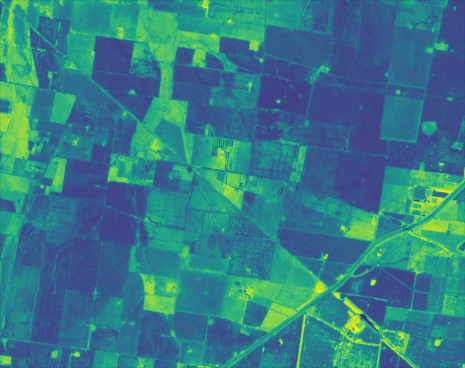
As a final step, we will just go through the image catalog we found, download our area of interest, and perform some local processing, which in this example will be just computing the NDVI and saving an image.

def plotNDVI(nir,red,filename):
    ndvi = (nir-red)/(nir+red)
    ndvi[ndvi>1] = 1
    plt.imshow(ndvi)
    plt.savefig(filename)
    plt.close()

Of course, in a real application we would be using much more advanced techniques, like image segmentation or machine learning. What I want to stress in the present guide, is that we can prototype those algorithms locally and later deploy them to the cloud (a topic we will cover in a subsequent post).

Now the only thing left is to loop over the catalog and process all the files, which we do as follows:

from rasterio.features import bounds
import matplotlib.pyplot as plt

bbox = bounds(geometry)

for i,item in enumerate(Sentinel_items):
    red_s3 = item.assets['B04']['href']
    nir_s3 = item.assets['B08']['href']
    date = item.properties['datetime'][0:10]
    print("Sentinel item number " + str(i) + "/" + str(len(Sentinel_items)) + " " + date)
    red = getSubset(red_s3, bbox)
    nir = getSubset(nir_s3, bbox)
    plotNDVI(nir,red,"sentinel/" + date + "_ndvi.png")

for i,item in enumerate(Landsat_items):
    red_s3 = item['assets']['red']['alternate']['s3']['href']
    nir_s3 = item['assets']['nir08']['alternate']['s3']['href']
    date = item['properties']['datetime'][0:10]
    print("Landsat item number " + str(i) + "/" + str(len(Landsat_items)) + " " + date)
    red = getSubset(red_s3, bbox)
    nir = getSubset(nir_s3, bbox)
    plotNDVI(nir,red,"landsat/" + date + "_ndvi.png")

Step 5: Deploy on an EC2 instance

After you finished testing, you might want to run your code directly on AWS. This will substantially reduce latency, and also give you access to more computing power.

After launching an EC2 instance and logging in, you will need to install the required dependencies like before. Assuming you are using an Amazon Linux 2 instance it should be straightfoward:

pip3 install sat-search pyproj rasterio[s3]

Now, an extremely simple way to deploy a Python script to an EC2 instance, is to upload it using scp.

scp -i security-key-file.pem sentinel-script.py ec2-user@ec2_elastic_ip:/home/ec2-user/

Running the script could result in the following error:

rasterio.errors.RasterioIOError: Illegal characters found in URL

This can hapened because we haven’t configured our EC2 instance to be able to access s3 buckets. See this video tutorial about how to do it the proper way (establishing suitable Roles in the IAM console). Note: you shouldn’t use aws configure and enter your credentials because that is a terrible from a security point of view.

Also, on Amazon Linux 2, the CA certificates where stored on a different location than my local computer, so after digging around a little, I found them:

os.environ['CURL_CA_BUNDLE'] = '/etc/ssl/certs/ca-bundle.crt'

After this, your Python code should run successfully.

Conclusion

Hopefully this tutorial has cleared out some basic questions and helped you get started with Cloud Optimized GeoTIFFs on AWS S3, using Python.

Remember that you can get the complete code for this tutorial here.

I plan to write more tutorials on Cloud-Native Geospatial Development. One way to get a notification whenever new content comes out is to subscribe to my mailing list (I only send one e-mail per month, at most).