Examples of Multiple Dispatch

Multiple dispatch and generic functions

One of most distinctive features of Julia is called multiple dispatch. While this is usually a topic that takes some time to fully understand and appreciate, the underlying concept is, in fact, quite simple.

In a few words, multiple dispatch is the possibility of having generic functions with multiple associated methods, each one for a different combination of argument types.

Note: Multiple dispatch is a generalization of single dispatch, where different methods are called based on the type of a single argument. For simplicity, we will first discuss examples of Julia’s dispatch system in the case of one-argument functions, as Julia has unique characteristics even in this case. Additionally, we will give an example of double dispatch at the end of the article.

A notion that is related to this idea of generic functions, is that of generic programming, which is a feature of a programming language which enables us to write programs in their most general and abstract form.

Generic programming is almost the default behavior in Julia. For example, let’s consider the following function:

f(x) = x^2

This function can be applied to integers, floats, complex numbers, and even matrices, without modifications.

We can also have functions that have multiple (different) methods depending on their input parameters. The language will determine which method to use (i.e. dispatch), when the function is called using specific argument types.

Let’s consider the following function definitions with type annotations:

f( x :: Int ) = "This is an Int: $(x)"
f( x :: Float64 ) = "This is a Float: $(x)"
f( x :: Any) = "This is a generic fallback"

f (generic function with 3 methods)

Here, Julia is telling us that the function f has 3 different methods associated with it. Calling f(1), f(1.5), and f("two") will execute the different definitions we have provided.

Note that, in the first two cases, Julia will be able to identify the input types and call the specialized functions we wrote. In the third case, as there is no specific function defined for type ‘String’, the third, generic function, will be executed.

Interestingly, we can use abstract types to define methods, for example:

f( x :: Number ) = "This is a Number: $(x)"

In Julia, we have both abstract and concrete types, and a hierarchy of types. For example, both the Int64 and Float64 types we have used are concrete types, and are both particular cases of the Number abstract type.

Now, the existence of a hierarchy of types enables Julia to call the most specific possible method which has been implemented, and rely on more generic methods otherwise. For example, let’s see what happens when we call our function using a complex floating-point number

f(1.2 + 3.5im)

"This is a Number: 1.2 + 3.5im"

There is a lot worth knowing about the type system, a topic which we might cover in future posts, but for now I will refer you to the official docs for further reading. Be warned that this is quite a thick topic.

Specializing an existing function for a new type

Let’s now consider the first of the use cases of multiple dispatch which we will discuss. Probably the most straightforward one is specializing a function, for example, for enhanced performance.

Let’s consider a very simple example. In mathematics, the gamma function is usually computed on the basis of several identities, or approximations. In Julia, we have the SpecialFunctions package which provides an implementation of the gamma function.

One of such identities is that, for integers, the gamma function reduces to the factorial function:

We can incorporate this identity by extending the gamma function implementation provided by SpecialFunctions, for the particular case of integers, as follows:

import SpecialFunctions:gamma
using BenchmarkTools

gamma( x :: Int ) = x > 0 ? factorial(x-1) : Inf

@btime gamma(15.0)      # 83.49 ns
@btime gamma(15)        # 1.81 ns

Interestingly, when we call the gamma function for the integer 15, the computing time is faster than when we call it for the floating-point number 15.0.

As a side note, the function we just wrote has overflow problems for integers larger than 21, so we can fallback to the floating-point values in such cases:

gamma( x :: Int ) = x > 0 && x < 21 ? factorial(x-1) : gamma(float(x))

Defining a new method for an existing type

We have just extended the definition of a function (gamma), for a new type (Int).

Interestingly, it turns out that we can also do the converse: take an existing type, and extend it with a new method.

For example, let’s consider the Triangle type provided by the package Meshes.jl. Let’s say we want to have a function that takes a given triangle and does something with it, like compute it’s barycentre. There is actually a quite simple formula for the barycentre $(x,y)_{\mathrm{centroid}}$:

using Meshes

barycenter( t :: Triangle ) = 
    Point([sum([ 1/3 *t.vertices[i].coords[j] for i in 1:3]) for j in 1:2])

And that’s it, we just added a new method to the Triangle type.

Now, we can use our new method as follows:

using MeshViz
import GLMakie as Mke

t = Triangle((0.,0.), (1.,1.), (0.,2.))
bary = barycenter(t)

viz(t)
viz!(bary,color=:red)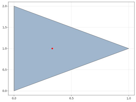

This might seem even too simple — and in fact, that’s the good news.

In object-oriented languages, extending a class defined in a third-party library is much more involved process. To do so, we have two options: we either have to convince the library authors to incorporate our code, or rely on inheritance, which results in a new derived class with a new name, which can cause troubles when attempting to reuse code.

Interface Design Example

So far we have only scratched the surface of what can be accomplished (and how conveniently!) by leveraging Julia’s dispatch system. There is a lot more to it, though.

Let’s consider another example of how Julia’s dispatch system can aid us in the creation of generic code in yet another way: by simplifying the design of an interface.

For instance, in the case of iterative solvers, we seek the solution the system

by only applying the matrix $A$ to different vectors. When using iterative solvers, we can either have the full matrix stored somewhere, or, instead, a functional representation of the matrix (i.e. the linear operator).

Let’s say we want to compute the largest eigenvalues of the following matrix:

n = 5
A = SymTridiagonal(2*ones(n),-ones(n-1))

5×5 SymTridiagonal{Float64, Vector{Float64}}:
  2.0  -1.0    ⋅     ⋅     ⋅ 
 -1.0   2.0  -1.0    ⋅     ⋅ 
   ⋅   -1.0   2.0  -1.0    ⋅ 
   ⋅     ⋅   -1.0   2.0  -1.0
   ⋅     ⋅     ⋅   -1.0   2.0

A functional representation of this matrix (of arbitrary size), is the following:

Afunc(x) = [2x[1] - x[2]; -x[1:end-2] + 2x[2:end-1] - x[3:end]; -x[end-1] + 2x[end]]

We would like to design an iterative solver which accepts both types of inputs.

The challenge here, is that this time, one of such inputs is an Array, and the other is a Function. These two objects are not different instances of an abstract type like before, they are totally different and unrelated types. So how can we do this?

Interestingly, multiple dispatch can help us achieve a high level of abstraction. For example, we can have code that works on anything which satisfies certain properties, pretty much like we do in mathematics.

Let’s move back to our problem to figure out which abstraction we need. Let’s remember that in the context of iterative solvers, we are not interested in a matrix per se, but in the linear operator defined by such matrix. An what can you do with a linear operator? You can apply it to vectors.

Therefore, we need to write code that could work for anything which has an associated apply function. We will call such object an operator.

This two lines suffice to create the interface we need:

apply( A :: Matrix, x ) = A*x
apply( f :: Function, x ) = f(x)

Now, let’s write a generic iterative solver, with an “operator” as an input argument. To keep it simple, we will code the power iteration method, which computes the largest eigenvalue and eigenvector of a given linear operator.

using LinearAlgebra

function PowerIteration( operator, dim, num_iters )
    bk = rand(dim)
    for iter ∈ 1:num_iters
        bk = apply(operator, bk)    # Here we apply A
        bk = bk / norm(bk)
    end
    λ = bk' * Afunc(bk) / (bk'*bk)
    return λ, bk
end

Now, the user of the above code can call this solver as follows:

λ, bk = PowerIteration(A, size(A,1), 25)
λ, bk = PowerIteration(Afunc, 5, 25)

This quite concise and elegant code.

Of course, there is more to interface design than what we have just discussed, but that should be the topic of another post.

Double dispatch and beyond

So far, we had been discussing examples of Julia’s dispatch system in the case of one-argument functions. However, unlike some other programming languages, Julia is not limited to dispatching on a single argument: it can dispatch on any finite number of arguments!

Of course the same principles apply. We can have functions of multiple arguments that specialize in particular cases, or we can extend existing types with functions of multiple arguments, all while avoiding extensive usage of if-else statements, and in a way which encourages modularity and code reuse.

Continuing with our example regarding Meshes.jl, we could consider operations like intersections and union, which take multiple geometrical shapes as parameters. So, if the package Meshes.jl didn’t provide those functions already, we could easily extend it, defining our own methods.

Additionally, let’s say that Meshes.jl implements a general routine for the intersection of polygons which is $O(n^2)$. And let’s assume that we happen to be in a case where we know that both of our polygons are convex, for which there is a specialized algorithm that requires $O(n)$ operations. We could then specialize the intersect function for such case with a this new algorithm, defining a function of the form:

intersect( S1 :: ConvexPolygon, S2 :: ConvexPolygon) = ... 

If we also make our ConvexPolygon a subtype of an abstract Geometry type implemented in Meshes.jl, then we don’t even need to write functions for the intersection of a ConvexPolygon with a Polygon (or a Polygon with a ConvexPolygon), as those calls would default to the already existing implementations of the intersect function, as a form of a generic callback.

As we see, the principles of ease of extensibility, modularity, and code reuse provided by Julia’s dispatch system are quite general features, that can be applied system-wide.

Summary: the multiple-dispatch paradigm

We just saw how Julia, being a dispatch-oriented language, allows us to combine custom types and methods in very flexible ways, with interesting applications.

It should be noted that similar functionality to what we have described can be also obtained in object-oriented languages. However, the resulting code will likely be more involved, requiring complicated definitions, the use of special syntax and/or keywords, and several extra lines of code. For example, in C++ we would need a combination of operator overloading, templates, and inheritance, to obtain something similar to what we have in Julia.

In sum, thanks to being carefully designed around multiple dispatch, the Julia language allows programmers to obtain a higher level of abstraction with substantially simpler code than competing alternatives, which should lead to higher levels of code reuse.

A related topic to multiple dispatch is the type system, which shall be the topic of a future post. Join the mailing list to get as soon as it comes out!